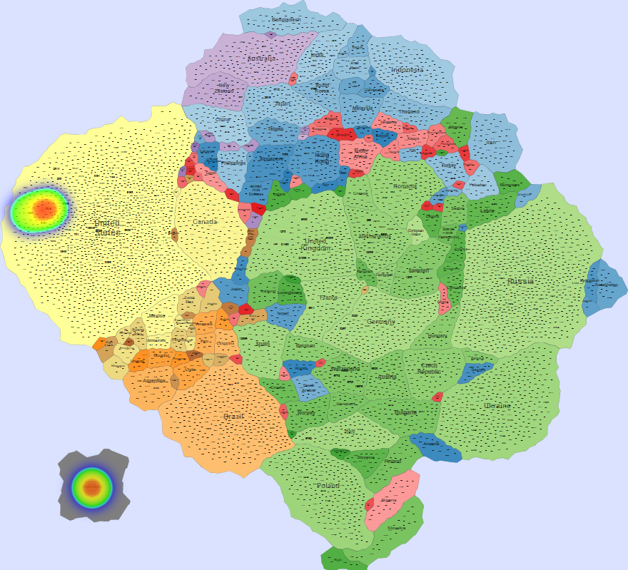
Paper and Supplemental Results

This page includes all the figures of the paper submitted to the Viszec'14.

We generate the following maps using the GMap framework [6], which produces geographical-like maps for a given graph. Using CAIDA data, we create an input graph where highly connected ASes are placed in closer positions. However, ASes belonging to the same country are moved from their initial positions into close proximity to avoid map
fragmentation [7].

Original image from paper
Full-sized image of the map used througout the experiment.
img/Scenarios_thumb/figure1_resize.png
Figure 1: Map of the AS topology with and without nodes and hot spots overlaid. Each country is shown as a contiguous region containing the ASes operating in their territory
img/Scenarios_thumb/figure3_resize.png
Figure 3: Topology map generated without applying the defragmentation step of Section 3.2.2.

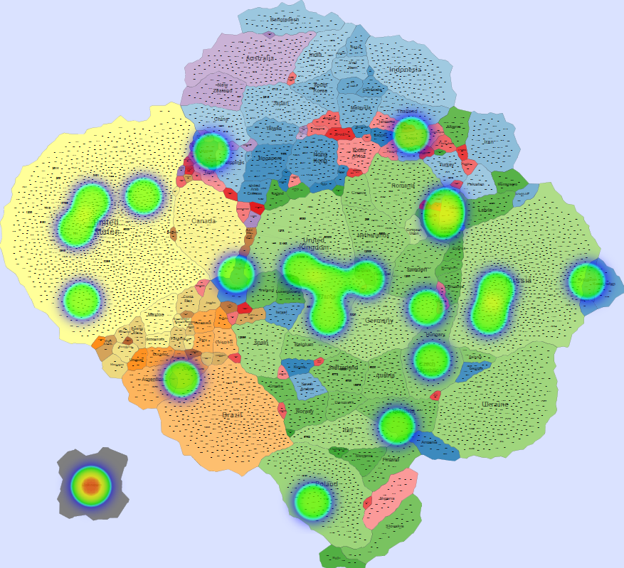
Two scenarios were created to demonstrate the usefulness of IMap. First, we use a sequence of heat maps to show the evolution of a DDoS attack. In the second scenario, we used real data [1] from a worm propagation event to study the origins of the worm and its propagation patterns. We used the CAIDA UCSD IPv4 Routed /24 Topology Dataset[2] to build the underlying AS topology in the IMap generation process.
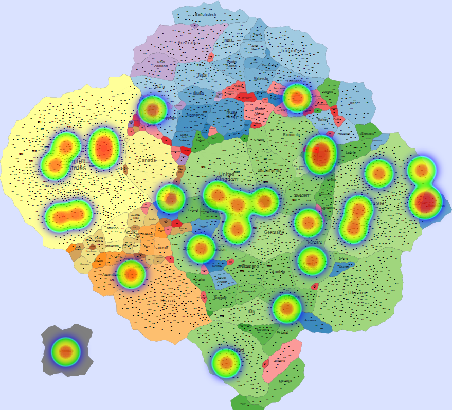
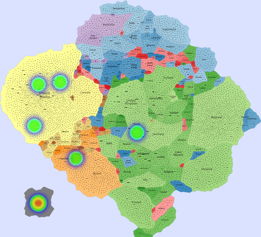
We generated synthetic DDoS attacks of varying intensity against a monitored network over a period of 25 minutes, using several attack topologies. Background traffic was generated by the D-ITG traffic generator[3] (100 random source IP nodes) and the DDoS attack (volumetric attack) was generated by the bonesi[4] package. The data rates from the DDoS hosts were greater than those generated by background traffic sources (in terms of the number of packets, volume, and number of IP flows). Composite metric C1 combines anomaly scores related to packet count and number of IP flows. Composite metric C2 combines anomaly scores related to traffic volume and number of IP flows (more details in GlobeCom 2014).
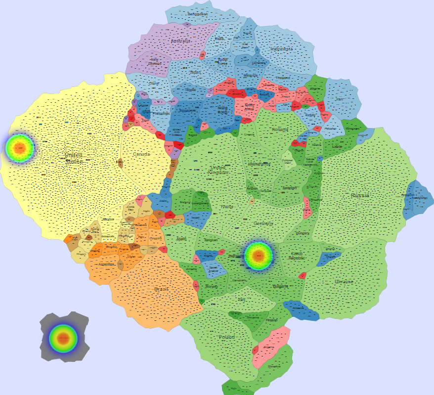
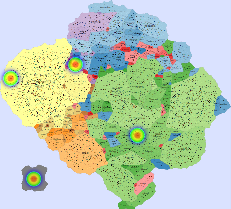
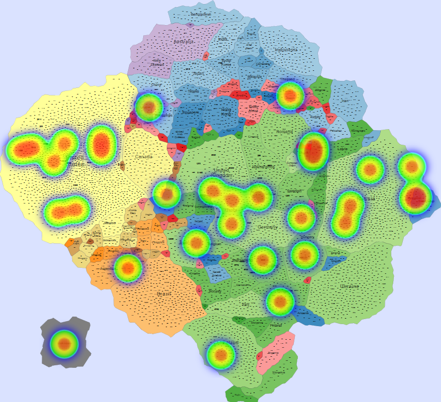
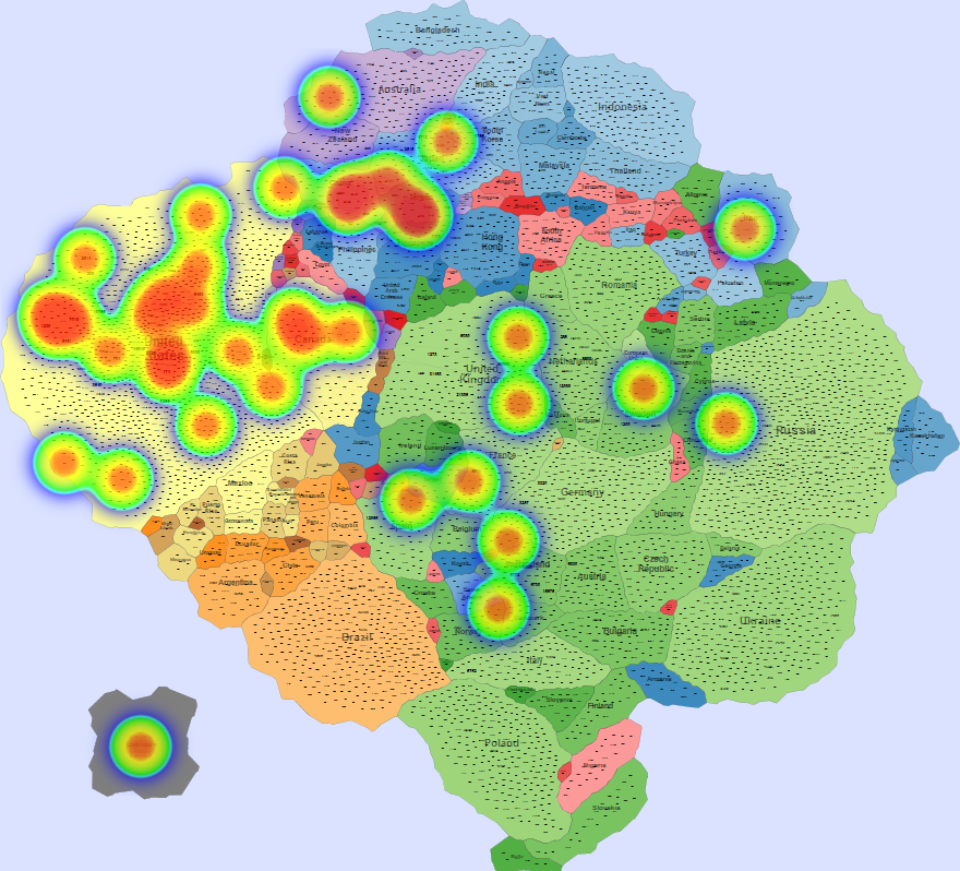
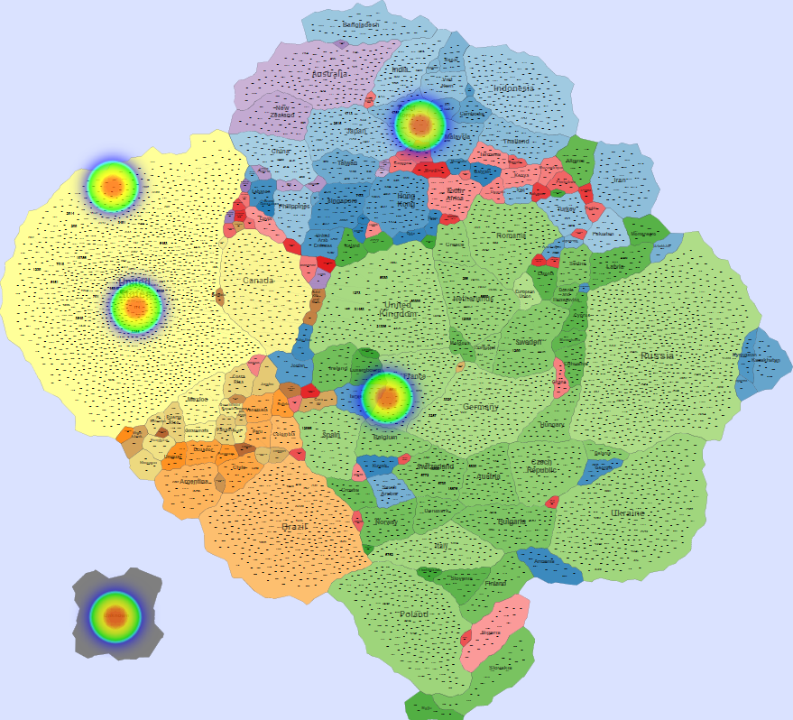
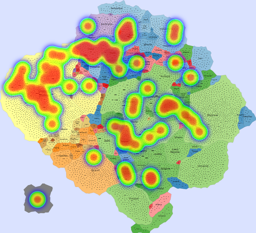
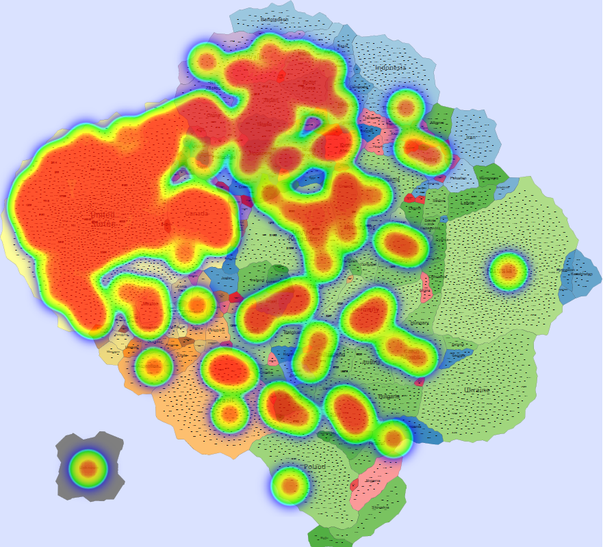
img/DDos_thumb/figure7a_resize.png
Figure 7a: DDoS attack, Interval 1, Metric C1
img/DDos_thumb/figure7b_resize.png
Figure 7b: DDoS attack, Interval 2, Metric C1
img/DDos_thumb/figure7c_resize.png
Figure 7c: DDoS attack, Interval 3, Metric c1. Botnet attack
img/DDos_thumb/figure7d_resize.png
Figure 7d: DDoS attack, Interval 4, Metric c1
img/DDos_thumb/figure7e_resize.png
Figure 7e: DDoS attack, Interval 5, Metric c1. Botnet attack
img/DDos_thumb/figure7f_resize.png
Figure 7f: DDoS attack, Interval 1, Metric C2
img/DDos_thumb/figure7g_resize.png
Figure 7g: DDoS attack, Interval 2, Metric C2
img/DDos_thumb/figure7h_resize.png
Figure 7h: DDoS attack, Interval 3, Metric C2. Botnet attack
img/DDos_thumb/figure7i_resize.png
Figure 7i: DDoS attack, Interval 4, Metric C2
img/DDos_thumb/figure7j_resize.png
Figure 7j: DDoS attack, Interval 5, Metric C2. Botnet attack

In July 19th, 2001, a variant of the Code-Red worm appeared and spread very rapidly around the world. The CAIDA Code-Red Worms dataset [1] contains packet headers collected from three different network monitors. In the animations provided by CAIDA [5], the worm spread is presented by heat maps overlaid on top of geographical maps. Their conclusion was that\physical and geographical boundaries are meaningless in the face of a virulent attack". We used one of the datasets containing the data relative to the nodes (IP addresses and their respective Autonomous System) that were observed to be transmitting the worm.

Animations can be seen here.

img/CodeRed Worm_thumb/figure8a_resize.png
Figure 8a: Worm initially spreads
img/CodeRed Worm_thumb/figure8b_resize.png
Figure 8b: Worm initially spreads
img/CodeRed Worm_thumb/figure8c_resize.png
Figure 8c: Reaches several countries at once
img/CodeRed Worm_thumb/figure8d_resize.png
Figure 8d: Propagates to several ASes within the same country
img/CodeRed Worm_thumb/figure8e_resize.png
Figure 8e: Attains the peak of activity

References

[1] CAIDA. Dataset on the code-red worms, 2001. http://www.caida.org/data/passive/codered_worms_dataset.xml.
[2] CAIDA. UCSD IPv4 routed /24 topology dataset, month of july, 2014. http://www.caida.org/datactive/ipv4_routed_24_topology_dataset.xml
[3] http://traffic.comics.unina.it/software/ITG
[4] http://code.google.com/p/bonesi
[5] J. Brown. Animations for code-red worms spread, 2001. http://www.caida.org/research/security/ code-red/coderedv2_analysis.xml#animations.
[6] E. R. Gansner, Y. Hu, and S. G. Kobourov. Visualizing Graphs and Clusters as Maps. In IEEE CGA, pages 2259-2267, 2010.
[7] S. G. Kobourov, S. Pupyrev, and P. Simonetto. Visualizing graphs as maps with contiguous regions. In EuroVis Short Papers, pages 31-35, 2014.